Models for Distributed Routing Protocols

Part 1: SIMPLE Models and Simulation

One of the keys to success of any verification effort is identifying a class of models capable of representing the important elements of the system under consideration. Such models inevitably elide information—the real world is too complicated to represent it in its entirety. However, a good model represents enough of the real world to be useful. When it comes to software reliability, such models need to represent the causes of important bugs or vulnerabilities.

For instance, relational algebra has been an effective model for database query languages for decades. It represents database tables as relations, which, mathematically speaking, are just sets of tuples, and is capable of defining a variety of standard database operations such as filters, joins and maps. It has been indispensable for helping database implementers define and prove correct complex query transformations and optimizations. Of course, there are infinitely many things that the (standard) relational algebra models will not capture about databases: the concrete syntax of user queries, the cost of computing filters or joins, or the semantics of the underlying storage system and its potential for failure, to name just a few.

The networking community, like the databases community, has its fair share of models as well. In this post, we will introduce a simple class of models that capture the essence of distributed routing protocols like eBGP, OSPF, RIP and ISIS. They describe the flow of routing messages between devices and allow us to analyze the routes (i.e., paths) computed by the network control plane, without getting bogged down by the bells and whistles of real-world protocols. The bells and whistles are important for practical reasons but have little bearing on a broad class of verification questions of interest such as: Does the network control plane compute a route from server A to server B? Might Google accidentally try to act as transport for traffic destined for Japan, possibly shutting off access to the internet there? Will Level 3 leak routes that should be kept internal, disrupting internet service across the US? By developing the capability to analyze these simple models, we can identify a range of potentially devastating errors in the configuration of modern networks.

The models we will discuss here are derived from the pioneering research of Griffin et al. [1] and Sobrinho [2]. Griffin identified the fact that network protocols like BGP are solving a kind of “stable paths problem”. In doing so, he developed a solid framework for thinking rigorously about such protocols and analyzing their basic properties, including convergence and determinacy. Sobrinho generalized these ideas and formalized them from an algebraic perspective. More recently, we developed NV [3, 4], a language and system that allows users to define and verify such models using powerful logical tools.

SIMPLE: An Idealized Control Plane Protocol

While there are many distributed control plane protocols, they share a common structure. That common structure allows us to define a wide range of protocols in the same way, and makes it possible to implement generic analysis tools that can be reused to find bugs in any of them.

To illustrate the basic pieces of a model, let’s take a look at a concrete example—a made-up protocol we will call SIMPLE. In SIMPLE, each router in the network either knows a route to the destination or it doesn’t. We use the symbol None to represent “no route.” Each known route is a triple (pref, length, next). The first component, pref, is a numeric preference for the route. The higher the number, the more desirable the route. In general, the reader can assume the protocol uses 32-bit numbers that range from $0$ to $2^{32}-1$, but the details do not matter. The second component is the length of the path to the destination. The third component identifies the router that serves as the next hop along the journey to the destination. For simplicity, SIMPLE is designed to route to a single destination, so we don’t need to include the name of the destination (i.e., its IP address) in the routing messages. We’ll discuss more elaborate models for multi-destination routing later in this series of articles. To summarize, we have now defined the first component of a control plane model, the set of messages M, that are used to disseminate routing information amongst routers.

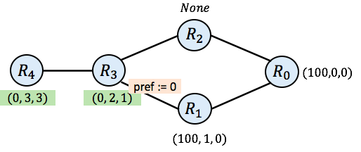
Below is an example of a network running SIMPLE in an initial state, before the process of computing routes to the destination has begun. This network has 5 routers, named $\mathtt{R_0} - \mathtt{R_4}$. Each router is annotated with an initial route. $\mathtt{R_0}$ is the destination router—its initial route has a preference of 100, a length of 0 to the destination (it is the destination), and a dummy next-hop of 0. The other routers have None as their initial route.

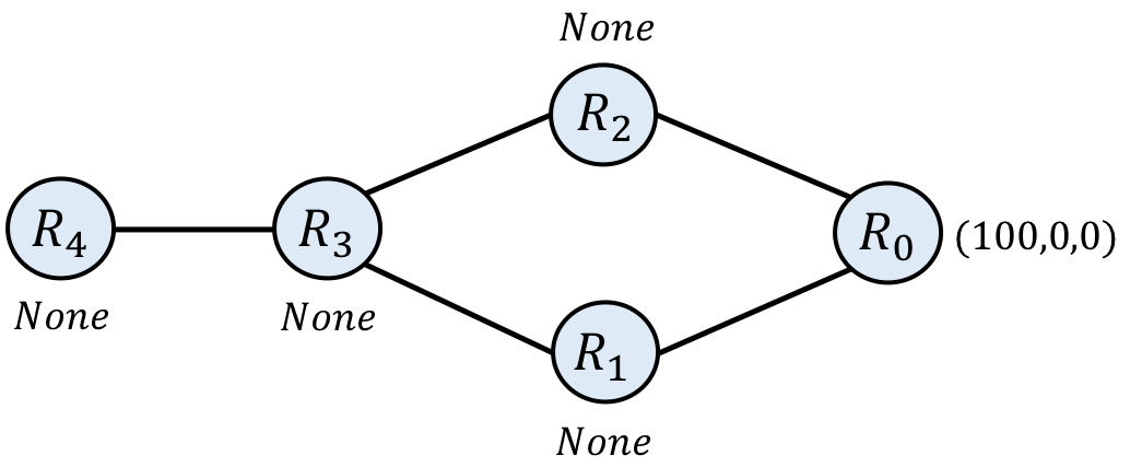
In general, the current state X of one of our network models is a function from routers to their current route. The initial state init, is an example of such a state. In this case, we define the init state for this network as follows:

$\mathtt{\mathbf{init}_{R}} = \mathtt{(100, 0, 0)}~~~,~\mathrm{if}~\mathtt{R} = \mathtt{R_0}$

$\mathtt{\mathbf{init}_{R}} = \mathtt{\mathit{None}}~~~,~\mathrm{otherwise}$

The routing process for SIMPLE, and other protocols we model, operates by transmitting messages around the network, and updating the network state as we go. Eventually (we hope), the process stabilizes and no more state changes occur.

Informally, SIMPLE operates as follows. Each router with a valid route can choose to export the route to one or more of its neighbors. When a message traverses an edge in the graph, it is transformed. The length of the route will increase by one, the next hop field will change, and the importer will change the preference field, making the route more or less desirable. We call the function that executes those transformations the trans function. Since the transformation may vary from one edge of the graph to the next, when we care to be specific, we write $\mathbf{\mathtt{trans}}_{\mathtt{e}}$ for the transformation function to be applied across the edge e.

When a router receives one or more routes from its neighbors, it compares those routes with its initial route and chooses the most desirable route available. More specifically, it prefers the route with the highest preference value. If there is a tie, it will prefer the route with the shortest path length. If there is still a tie, it prefers the route through the lowest numbered neighbor (e.g., all other things being equal, router $\mathtt{R_3}$ prefers routes it receives from $\mathtt{R_1}$ over those it receives from $\mathtt{R_2}$). In general, when multiple routes are available at a router, the router will use information from those routes to compute its most desired route. We call the function that executes that computation the merge function, and often write $\mathtt{R_1~+~R_2}$ to denote the merge of two routes, $\mathtt{r_1}$ and $\mathtt{r_2}$. In principle, the merge function can differ at every router. If we care to distinguish between the merge functions of particular routers, we will write merge$_R$, or $\mathtt{R_1}~\mathtt{+_R}~\mathtt{R_2}$, for the merge at router R, but to keep the notation light, we will often assume the merge functions are the same across all nodes and elide the subscript.

Choices such as which router forwards routes to which other routers, and how to change a field like the preference value are typically part of the configuration of a protocol. In contrast, the notion of “most desirable route” (i.e., the merge function) is usually a fixed part of the protocol. The configurations are typically defined by network operators—they are what allows a protocol to be customized to the needs of a particular network. Router vendors like Cisco and Juniper have complex, proprietary languages for configuring their devices, and in large networks, such configurations can be hundreds or thousands of lines of code per router, and hundreds of thousands or millions of lines in total for a large data center network. However, when it comes to network verification, it does not really matter whether a route processing function is defined by a configuration or is an inherent, unchangeable part of the protocol. Hence, our models incorporate both and do not distinguish between fixed and configurable parts.

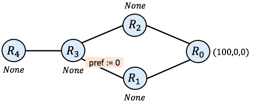
In the following picture, we add a little bit of configuration information to our network. In particular, we will assume that when $\mathtt{R_3}$ imports a message from $\mathtt{R_1}$ it changes the preference value to 0, making it less desirable than routes imported from $\mathtt{R_2}$. We can also configure the network so that certain links drop messages. For simplicity, we will assume links propagate messages from right to left, and drop all messages (i.e., producing None) from left to right.

Protocol Simulation

To determine which paths each router in the network chooses to use, we can simulate execution of the control plane protocol on the given network. Simulation updates the network state, one step at a time until a “stable state” is found and no more updates are required. The following (non-deterministic) algorithm implements the simulation process.

Generic Simulation Algorithm

1. Let X, the current state of the simulation, be the initial state init.

2. Select any router R:

   • Let $\mathtt{R_1} \ldots \mathtt{R_k}$ be the neighbors of R
   • Let $\mathtt{e_1} \ldots \mathtt{e_k}$ be the edges that connect those neighbors to R
   • Update X(R) as follows (leaving other components of X unchanged):
     • $\mathtt{X}(\mathtt{R}) := \mathbf{\mathtt{trans}}_{\mathtt{e1}}(\mathtt{X}(\mathtt{R_1}))~\mathtt{+_R}~\ldots~\mathtt{+_R}~\mathbf{\mathtt{init}}(\mathtt{R})$

Repeat step 2 until there are no further changes to be made.
i.e., until $\mathtt{X}(\mathtt{R}) = \mathbf{\mathtt{trans}}_{\mathtt{e1}}(\mathtt{X}(\mathtt{R_1}))~\mathtt{+_R}~\ldots~\mathtt{+_R}~\mathbf{\mathtt{init}}(\mathtt{R})$for all routers R

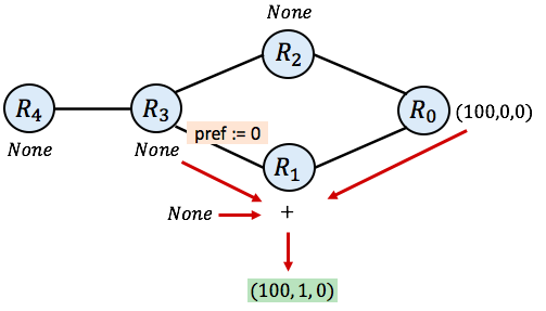
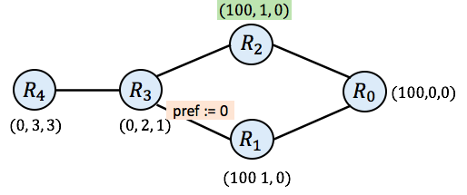
In our SIMPLE network, a possible first step in simulation could select router R1 and consider its neighbors, $\mathtt{R_3}$ and $\mathtt{R_0}$. The current chosen routes for those routers are None and (100, 0, 0) respectively. The initial route at $\mathtt{R_1}$ is None. Hence, the new route chosen by $\mathtt{R_1}$ after this step in simulation will be:

$\mathtt{\mathbf{trans}_{01}}(100,0,0) ~\mathtt{+}$

$\mathtt{\mathbf{trans}_{31}}(\mathtt{None})~\mathtt{+}$

$\mathtt{None}$

which is equal to the following (we add 1 to the length of the known route and leave the other fields unchanged):

$(100, 1, 0) ~\mathtt{+}~ \mathit{None} ~\mathtt{+}~ \mathit{None}$

which is equal to

$(100, 1, 0)$

as the SIMPLE protocol always prefers some route over None. The following picture diagrams the process. The green route is the route that emerges for $\mathtt{R_1}$ after a single step of simulation:

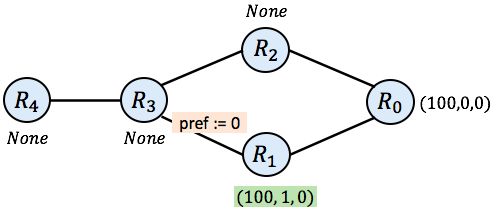
Cleaning up the picture, our network now looks like this:

Next, it may be $\mathtt{R_3}$’s turn to act. As mentioned above, when $\mathtt{R_3}$ imports its message from $\mathtt{R_1}$, it downgrades the preference to 0. However, since $\mathtt{R_3}$ only receives None (no route yet) from $\mathtt{R_2}$, it prefers the low-preference route from $\mathtt{R_1}$ over no route at all. After $\mathtt{R_3}$, $\mathtt{R_4}$ may take a turn, leaving the network in the following state after those two steps:

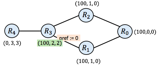
And then the simulation might choose to update $\mathtt{R_2}$:

And now you will notice that all routers have a valid route (none of the routers have None as their route). Still, the simulation is not complete. If router $\mathtt{R_3}$ goes again at this point, it will compute the new route (100, 2, 2), which differs from its current route of (0, 2, 1). It does so because SIMPLE prefers routes with higher preference value. As a result, $\mathtt{R_3}$ prefers the route it receives from $\mathtt{R_2}$ (with preference 100) rather than the route it received earlier from $\mathtt{R_1}$ (with preference 0). $\mathtt{R_3}$’s next hop is now 2 instead of 1.

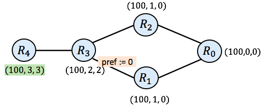
And then finally, we need to consider $\mathtt{R_4}$ again. When $\mathtt{R_4}$ pulls routes from all its neighbors now, we arrive in the following state.

Model Solutions

At this point, we can examine all routers R and check to see whether the current chosen route equals $\mathbf{\mathtt{trans}}_1(\mathtt{r_1}) \mathtt{+_R} \ldots \mathtt{+_R} \mathbf{\mathtt{trans}}_k(\mathtt{r_k}) \mathtt{+_R} \mathbf{\mathtt{init}}(\mathtt{R})$ where $\mathtt{r_1}$ through $\mathtt{r_k}$ are the current routes of R’s neighbors. It turns out they all do.

(Aside: Recall that we specified that edges, when traversed from left to right, drop all routes—that is, they convert any route from left to right into None—and so the route with higher local preference of 100 at $\mathtt{R_3}$ does not propagate backwards to $\mathtt{R_1}$. If we did not block this route, the system would not yet be stable.)

So we’ve reached a stable state of the system, which we also call a solution to the routing system. More formally, a solution L is any state of a network that is globally stable in the sense that all routers R satisfy the following equation:

$\mathbf{\mathtt{L}}(\mathtt{R}) = \mathbf{\mathtt{trans}}_{\mathtt{e1}}(\mathbf{\mathtt{L}}(\mathtt{R_1})) \mathtt{+_R} \ldots \mathtt{+_R}~\mathbf{\mathtt{init}}(\mathtt{R})$

where

• $\mathtt{R_1}, \ldots, \mathtt{R_k}$ are the neighbors of R
• $\mathtt{e_1}, \ldots, \mathtt{e_k}$ are the edges connecting those neighbors to R

Once we have a solution, we can examine its properties. For instance, given a solution L, we could ask whether L(R) = None for any router R, indicating that that router receives no route from the destination and hence cannot reach it. We could also ask what the length of the longest path from any node to the destination is. By using the next-hop fields of routes, we can also reconstruct the path that any router uses to reach the destination. If we were concerned with a property of that path, such as whether it traverses a particular waypoint (like $\mathtt{R_2}$ or $\mathtt{R_1}$) then we could deduce that as well.

Summary

Routing is the process of computing paths to a given destination or a collection of destinations. There are many different distributed routing protocols that engage in this process; they go by names such as BGP, OSPF, ISIS and others.

It turns out these protocols have a lot of structure in common. We can see that commonality by defining a class of models with the components (G, M, trans, merge, init):

• G — A graph representing the topology of the network (with vertices V and edges E).

• M — The set M of messages, also called routes, used by the protocol.

• trans : E → M → M — The function that propagates, transforms or discards messages/routes as they travel across each edge in the network.

• merge : V → M → M → M — The function that combines incoming information from neighboring routers, usually selecting one (or more) most preferred route for traffic traveling to the given destination.

• init : V → M — The initial routes (init) at each node in the graph, which are used in the absence of receiving additional information about where or how to route traffic.

Given these components, we have enough information to simulate a model and find its solution, or stable state. And once we have a solution in hand, we can analyze it to determine what sorts of properties it has. For instance, we can determine whether a given router can reach a particular destination, or whether a computed route passes through a particular waypoint. Such properties can help us uncover important bugs in network configurations before they are deployed.

There’s a lot more to learn about this topic, and in future blog posts, we will explore some of them. Can a system have more than one solution? How can we tell? Are there algorithms for finding them all? What happens when there are failures? Can we reason about quantitative properties like congestion? How do we construct models of real protocols like BGP, OSPF and their interactions? How does one actually implement network simulation and verification tools based on these models?

References

[1] The stable paths problem and interdomain routing. T. G. Griffin, F. B. Shepherd, G. Wilfong. IEEE/ACM Transactions on Networking 10(2). April 2002. https://ieeexplore.ieee.org/document/993304

[2] An algebraic theory of dynamic routing. J. L. Sobrinho. IEEE/ACM Transactions on Networking 13(5). Oct 2005. https://ieeexplore.ieee.org/document/1528502

[4] NV: Tools for modeling and analyzing network configurations. June 2020. https://github.com/NetworkVerification https://github.com/NetworkVerification/nv

[5] NV: An Intermediate Language for Verification of Network Control Planes. Nick Giannarakis, Devon Loehr, Ryan Beckett and David Walker. ACM SIGPLAN Conference on Programming Language Design and Implementation (PLDI). June 2020. https://www.cs.princeton.edu/~dpw/papers/nv-pldi20.pdf